Basic usage
This example provides an minimal overview of Slitflow by analyzing the trajectories of simulated random walks.
1. Installation
You can run the example in the cloud using Gitpod or Google Colaboratory in your web browser without installing Slitflow on your computer.
You can also run the example on your local Windows, Linux, or Mac computer by executing the Python script or using Jupyter notebook after installing Slitflow.
In the cloud
If you have a Google account, you can run the example in Google Colaboratory. Click the following badge to launch the Jupyter notebook.
If you have a GitHub account, you can run the example in Gitpod. Follow these steps (some may be skipped if you’ve run it before):
Open the slitflow repository on Gitpod.
Click
Continue with GitHuband sign in to authorize Gitpod.On the
New Workspacepage, clickContinue.The environment will be set up automatically, and the VS Code editor will launch.
Open the file
scripts/getting_started_basic.pyand click theRun Python Filebutton located at the top right of the editor.
Windows 10/11
Install Slitflow locally by following these steps using virtual environment and pip:
Install the latest Python 3.8, 3.9 or 3.10 from Python.org.
Create a virtual environment using venv.
Activate the virtual environment and run
pip install slitflowto install the minimal functionality of Slitflow.Download the example Python script and execute it.
macOS
The following steps are tested on macOS Ventura 13. Installing ttf-mscorefonts-installer
is recommended to reproduce the figures.
Install the latest Python 3.8, 3.9 or 3.10 using pyenv.
Create virtual environment using pyenv-virtualenv.
After activating the virtual environment, execute the
pip install slitflowcommand to install the minimal functionality of Slitflow.Download the example Python script and execute it.
Linux
The following steps are tested on Ubuntu 22.04.1.
Install the latest Python 3.8, 3.9 or 3.10 using pyenv.
Create virtual environment using pyenv-virtualenv.
After activating the virtual environment, execute the
pip install slitflowcommand to install the minimal functionality of Slitflow.Download the example Python script and execute it.
2. Preparing tutorial directory
In the latter part of the Basic tutorial (3.4), the results of each analysis step are stored in the project directory. To create the project directory in your workspace, follow these steps.
import os

root_dir = "slitflow_tutorial"
project_dir = os.path.join(root_dir, "getting_started_basic")

# Create directories
if not os.path.isdir(root_dir):
    os.makedirs(root_dir)
if not os.path.isdir(project_dir):
    os.makedirs(project_dir)
3. Running the example
We usually import slitflow as follows:
import slitflow as sf
3.1. Simulate random walks
Start by creating an Index object that defines the number of images and
trajectories. Then we execute the run() method to make result data inside
the Index object.
See also slitflow.tbl.create.Index for argument descriptions.
D1 = sf.tbl.create.Index()
D1.run([], {"type": "trajectory", "index_counts": [2, 3], "split_depth": 0})
print(D1.data[0])
#   img_no trj_no
# 0      1      1
# 1      1      2
# 2      1      3
# 3      2      1
# 4      2      2
# 5      2      3
Then we append random walk coordinates to the index table by making the next analysis object.
See also slitflow.trj.random.Walk2DCenter for argument descriptions.
D2 = sf.trj.random.Walk2DCenter()
D2.run([D1], {"diff_coeff": 0.1, "interval": 0.1, "n_step": 5, "length_unit": "um", "seed": 1, "split_depth": 0})
print(D2.data[0])
#    img_no  trj_no  frm_no      x_um      y_um
# 0        1       1       1  0.000000  0.000000
# 1        1       1       2  0.229717 -0.325487
# 2        1       1       3  0.143202 -0.078733
# 3        1       1       4  0.068507 -0.186384
# 4        1       1       5 -0.083234 -0.141265
# ...
# 34       2       3       5 -0.218346  0.373677
# 35       2       3       6 -0.247888  0.498855
3.2. Calculate the Mean Square Displacement
The following code calculates the MSD of each trajectory. Then MSDs are averaged through all images.
See also slitflow.trj.msd.Each and slitflow.tbl.stat.Mean.
D3 = sf.trj.msd.Each()
D3.run([D2], {"group_depth": 2, "split_depth": 0})

D4 = sf.tbl.stat.Mean()
D4.run([D3], {"calc_col": "msd", "index_cols": ["interval"], "split_depth": 0})
print(D4.data[0])
#    interval       msd       std       sem  count       sum
# 0       0.0  0.000000  0.000000  0.000000      6  0.000000
# 1       0.1  0.034335  0.014093  0.005754      6  0.206012
# 2       0.2  0.065532  0.023673  0.009665      6  0.393195
# 3       0.3  0.116515  0.031346  0.012797      6  0.699089
# 4       0.4  0.138391  0.066066  0.026971      6  0.830347
# 5       0.5  0.153488  0.112978  0.046123      6  0.920926
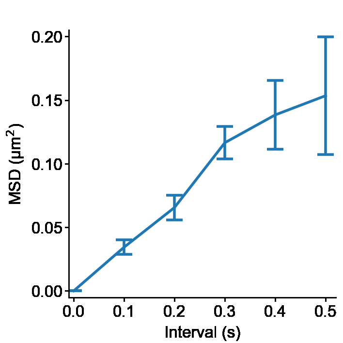
3.3. Make a figure image
Then plot the averaged MSD against the time interval. The graph style is adjusted using style class and creates a figure tiff image.
See also slitflow.fig.line.Simple, slitflow.fig.style.Basic and slitflow.fig.figure.ToTiff
Note
By default, Slitflow disables the display of figures in a separate window using Matplotlib. If your environment allows a separate window display, include the following snippets in your Python script after importing slitflow.
import matplotlib
matplotlib.use('TkAgg')
import matplotlib.pyplot as plt

D5 = sf.fig.line.Simple()
D5.run([D4], {"calc_cols": ["interval", "msd"], "err_col": "sem", "group_depth": 0, "split_depth": 0})

D6 = sf.fig.style.Basic()
D6.run([D5], {"limit": [-0.01, 0.52, -0.005, 0.205], "tick": [[0, 0.1, 0.2, 0.3, 0.4, 0.5], [0, 0.05,
      0.1, 0.15, 0.2]], "label": ["Interval (s)", "MSD (\u03bcm$^{2}$)"], "format": ['%.1f', '%.2f']})

D7 = sf.fig.figure.ToTiff()
D7.run([D6], {"split_depth": 0})

plt.close()
plt.imshow(D7.to_imshow(0))
plt.axis("off")
plt.show()
3.4. Run using a pipeline
The Pipeline class can perform all the above steps while saving data to a project folder.
PL = sf.manager.Pipeline(project_dir)
obs_names = ["Sample1"]
PL.add(sf.tbl.create.Index(), 0, (1, 1), 'channel1', 'index',
      obs_names, [], [],
      {"type": "trajectory", "index_counts": [2, 3], "split_depth": 0})
PL.add(sf.trj.random.Walk2DCenter(), 0, (1, 2), None, 'trj',
      obs_names, [(1, 1)], [0],
      {"diff_coeff": 0.1, "interval": 0.1, "n_step": 5, "length_unit": "um", "seed": 1, "split_depth": 0})
PL.add(sf.trj.msd.Each(), 0, (1, 3), None, 'msd',
      obs_names, [(1, 2)], [0],
      {"group_depth": 2, "split_depth": 0})
PL.add(sf.tbl.stat.Mean(), 0, (1, 4), None, 'avemsd',
      obs_names, [(1, 3)], [0],
      {"calc_col": "msd", "index_cols": ["interval"], "split_depth": 0})
PL.add(sf.fig.line.Simple(), 0, (1, 5), None, 'msd_fig',
      obs_names, [(1, 4)], [0],
      {"calc_cols": ["interval", "msd"], "err_col": "sem", "group_depth": 0, "split_depth": 0})
PL.add(sf.fig.style.Basic(), 0, (1, 6), None, 'msd_style',
      obs_names, [(1, 5)], [0],
      {"limit": [-0.01, 0.52, -0.005, 0.205], "tick": [[0, 0.1, 0.2, 0.3, 0.4, 0.5], [0, 0.05, 0.1, 0.15, 0.2]],
      "label": ["Interval (s)", "MSD (\u03bcm$^{2}$)"], "format": ['%.1f', '%.2f']})
PL.add(sf.fig.figure.ToTiff(), 0, (1, 7), None, 'msd_img',
      obs_names, [(1, 6)], [0],
      {"split_depth": 0})
PL.save("pipeline")
PL.run()
This code creates the following folder structure.
slitflow_tutorial/getting_started_basic
   |--g0_config
   |    pipeline.csv
   |--g1_groupe1
       |--a1_index
       |    Sample1_index.csv
       |    Sample1_index.sf
       |    Sample1_index.sfx
       |--a2_trj
       |    Sample1_trj.csv
       |    Sample1_trj.sf
       |    Sample1_trj.sfx
       |--a3_msd
       |    Sample1_msd.csv
       |    Sample1_msd.sf
       |    Sample1_msd.sfx
       |--a4_avemsd
       |    Sample1_avemsd.csv
       |    Sample1_avemsd.sf
       |    Sample1_avemsd.sfx
       |--a5_msd_fig
       |    Sample1_msd_fig.fig
       |    Sample1_msd_fig.sf
       |    Sample1_msd_fig.sfx
       |--a6_msd_style
       |    Sample1_msd_style.fig
       |    Sample1_msd_style.sf
       |    Sample1_msd_style.sfx
       |--a7_msd_img
            Sample1_msd_img.tif
            Sample1_msd_img.sf
            Sample1_msd_img.sfx
We can use the make_flowchat() method of the pipeline object to create an analytical flowchart diagram. The image is created as a PNG file in the g0_config folder in the project directory.
PL.make_flowchart("pipeline", "grp_ana")
