Advanced usage

This tutorial demonstrates a workflow of state-of-the-art analyses using single-molecule fluorescence movies in living cells.

1. Background

This example uses live-cell single-molecule movies of RNA polymerase II—that is, Pol II, a transcriptional protein complex—from cultured cells. Human U2OS cells expressing Halo-RPB1—the largest subunit of Pol II labeled with a self-labeling HaloTag—were stained with 3 nM Janelia Fluor fluorescence substrate, and excited using HILO illumination. 300 frames were captured at 33.33 ms per frame using an EMCCD camera.

This tutorial uses the wrapping classes of Python packages, including trackpy, fastspt, and tramway. Please consider citing the following references if the classes are helpful for your research.

[1] Allan DB, Caswell T, Keim NC, van der Wel CM, Verweij RW. soft-matter/trackpy: Trackpy v0.5.0 2021.

[2] Hansen AS, Woringer M, Grimm JB, Lavis LD, Tjian R, Darzacq X. Robust model-based analysis of single-particle tracking experiments with Spot-On. Elife 2018;7.

[3] Laurent F, Verdier H, Duval M, Serov A, Vestergaard CL, Masson J-B. TRamWAy: mapping physical properties of individual biomolecule random motion in large-scale single-particle tracking experiments. Bioinformatics 2022;38:3149–50.

2. Installation

If you have a GitHub account, you can run the example in Gitpod. You can also run the example on your local machine.

In the cloud

If you have a Google account, you can run the example in Google Colaboratory. Click the following badge to launch the Jupyter notebook.

If you have a GitHub account, you can run the example in Gitpod. See Installation for basic usage for details. Then, open the file scripts/getting_started_advanced.py and click the Run Python File button.

On your local machine

Additional Python packages are required for this tutorial. Please install them using one of the provided pip commands.

# If you want to install all the packages at once
pip install slitflow[full] git+https://gitlab.com/yumaitou/Spot-On-cli.git@py310

# If you downloaded requirements-full.txt from the slitflow repository
pip install -r requirements-full.txt

# If you want to install the packages manually
pip install trackpy tramway git+https://gitlab.com/yumaitou/Spot-On-cli.git@py310

Note

The original fastspt version installed from PyPI has a Python 3.10 environment error related to the version file during package import. For a temporary solution, a modified version of fastspt can be obtained from the forked repository.

Note

Trackpy package may require Visual Studio 2008 C++ runtime in certain environments. Please install the appropriate version from the microsoft website for your PC.

3. Downloading data and making a directory

To download image data of single-molecule movies (142 MB), get the zip file from zenodo. Unzip the file outside the project directory. In this tutorial, we assume the data is located in the slitflow_tutorial/data/getting_started_advanced directory in the user home directory. Use the script below to create directories and download the dataset.

import os
import urllib.request
import zipfile
import io

root_dir = "slitflow_tutorial"
project_dir = os.path.join(root_dir, "getting_started_advanced")
data_root_dir = os.path.join(root_dir, "data")
data_dir = os.path.join(data_root_dir, "getting_started_advanced")

# Create directories
if not os.path.isdir(root_dir):
    os.makedirs(root_dir)
if not os.path.isdir(project_dir):
    os.makedirs(project_dir)
if not os.path.isdir(data_root_dir):
    os.makedirs(data_root_dir)
if not os.path.isdir(data_dir):
    os.makedirs(data_dir)

# Download single-molecule movies

file_url = 'https://zenodo.org/record/7645485/files/getting_started_advanced.zip'

opener = urllib.request.build_opener()

# If you are in proxy environment, uncomment the following lines. Replace your_proxy_url and port with your proxy server.
# proxy_handler = urllib.request.ProxyHandler({
#     'https': 'your_proxy_url:port'})
# opener = urllib.request.build_opener(proxy_handler)

print("Downloading single-molecule movies. This may take tens of minutes.")
with opener.open(file_url) as download_file:
    with zipfile.ZipFile(io.BytesIO(download_file.read())) as zip_file:
        zip_file.extractall(data_root_dir)
print("Download completed.")

4. Running the example

We usually import slitflow as follows:

import slitflow as sf

4.1. Import movies

The image data are assumed to be stored in the slitflow/data directory in your home directory. The script below loads single-molecule movies, mask images of cell nuclei, and the parameter CSV file.

PL = sf.manager.Pipeline(project_dir)

pitch = 0.0710837445886793  # [um/pix]
interval = 0.03333  # [s]

for i in [1, 2, 3]:
    path = os.path.join(data_dir, "rpb1", "rpb1-" + str(i) + ".tif")
    PL.add(sf.load.tif.SplitFile(), 0, (1, 1), "rpb1", "raw",
           ["RPB1"], [], [],
           {"path": path, "length_unit": "um", "pitch": pitch,
            "interval": interval, "value_type": "uint8", "indexes": [i],
            "split_depth": 1})

path = os.path.join(data_dir, "mask", "mask.tif")
PL.add(sf.load.tif.SingleFile(), 0, (2, 1), "mask", "raw",
       ["RPB1"], [], [],
       {"path": path, "length_unit": "um", "pitch": pitch,
        "value_type": "uint8", "split_depth": 1})
PL.save("pipeline_1_load")
PL.run()

4.2. Tracking

Single-molecule tracking requires pre-processing and tracking algorithms that are appropriate for the characteristics of the acquired images. Here, we implemented a multistep customized process that focused on improving the location accuracy and processing time.

First, fluorescent spots were detected using a Difference of Gaussian filter and the local maximum—as used in u-track and TrackMate —and then selected using a cell nucleus region mask and an intensity threshold. The positions were further refined by 2D Gaussian fitting using a scipy.optimize.curve fit, the trajectories being extracted using the link function of Trackpy. To exclude noise trajectories, those with at least nine steps were selected.

These processes can be executed using the following pipeline script.

PL = sf.manager.Pipeline(project_dir)

PL.add(sf.img.filter.DifferenceOfGaussian(), 3, (1, 2), None, "dog",
       ["RPB1"], [(1, 1)], [2],
       {"wavelength": 0.6, "NA": 1.4, "split_depth": 1})
PL.add(sf.img.filter.LocalMax(), 3, (1, 3), None, "localmax",
       ["RPB1"], [(1, 2)], [2], {"split_depth": 1})
PL.add(sf.loc.convert.LocalMax2Xy(), 3, (1, 4), None, "xy",
       ["RPB1"], [(1, 3)], [2], {"split_depth": 1})
PL.add(sf.loc.mask.BinaryImage(), 2, (1, 5), None, "mask",
       ["RPB1"], [(1, 4), (2, 1)], [1, 1], {"split_depth": 1})
PL.add(sf.tbl.filter.CutOffPixelQuantile(), 2, (1, 6), None, 'cutoff',
       ["RPB1"], [(1, 5)], [2],
       {"calc_col": "intensity", "cut_factor": 4, "split_depth": 1})
PL.add(sf.loc.fit.Gauss2D(), 3, (1, 7), None, 'refine',
       ["RPB1"], [(1, 1), (1, 6)], [2, 2],
       {"half_width": 4, "split_depth": 1})
PL.add(sf.trj.wtrackpy.Link(), 3, (1, 8), None, 'trj',
       ["RPB1"], [(1, 7)], [1], {"search_range": 0.8, "split_depth": 1})
PL.add(sf.trj.filter.StepAtLeast(), 2, (1, 9), None, 'long',
       ["RPB1"], [(1, 8)], [1],
       {"step": 9, "group_depth": 2, "split_depth": 1})
PL.add(sf.tbl.math.Centering(), 1, (1, 10), None, "center",
       ["RPB1"], [(1, 9)], [1],
       {"calc_cols": ["x_um", "y_um"], "group_depth": 1, "split_depth": 1})
PL.save("pipeline_2_tracking")
PL.run()

The first three processes can be replaced with slitflow.loc.convert.LocalMax2XyWithDoG to reduce calculation time and file size.

Since this strategy is just one example, you can customize the pipeline to suit the feature of images and the behavior of target molecules.

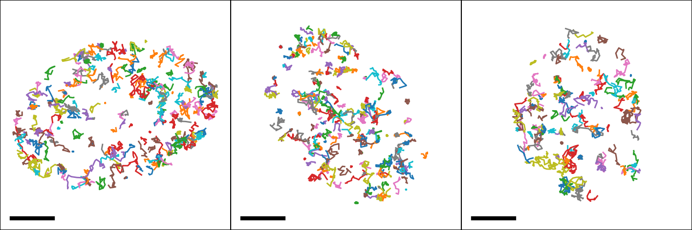
4.3. Show trajectory

The following pipeline creates the trajectory image for each cell nucleus.

PL = sf.manager.Pipeline(project_dir)

PL.add(sf.fig.line.Simple(), 2, (3, 1), "show", "fig",
       ["RPB1"], [(1, 10)], [1],
       {"calc_cols": ["x_um", "y_um"], "group_depth": 2, "split_depth": 1})
PL.add(sf.fig.style.Basic(), 2, (3, 2), None, "style",
       ["RPB1"], [(3, 1)], [1],
       {"size": [4, 4], "margin": [0, 0, 0, 0],
       "limit": [-14, 14, -14, 14], "tick": [[-15, 15], [-15, 15]],
        "is_box": True, "line_widths": 0.7,
        "split_depth": 1})
PL.add(sf.fig.figure.ToTiff(), 2, (3, 3), None, "tif",
       ["RPB1"], [(3, 2)], [1],
       {"scalebar": [5, 0.05, 0.05, 2, [0, 0, 0]],
       "dpi": 300, "split_depth": 0})
PL.add(sf.img.montage.RGB(), 0, (3, 4), None, "mtg",
       ["RPB1"], [(3, 3)], [0],
       {"grid_shape": [1, 3], "padding_width": 0, "split_depth": 0})
PL.save("pipeline_3_show_trajectory")
PL.run()

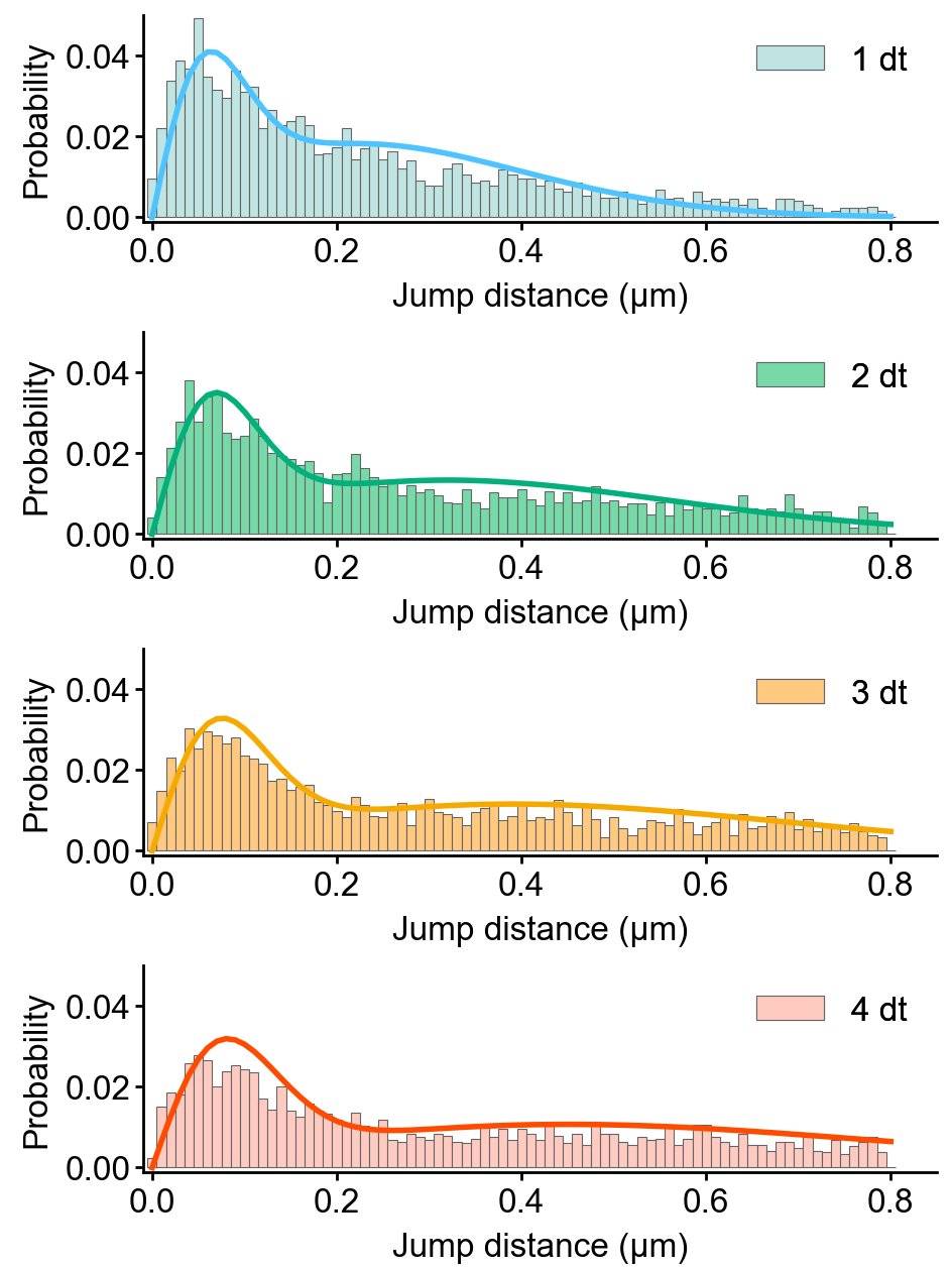
4.4. Spot-On analysis

Spot-On is state-of-the-art kinetic modeling of single particle trajectories (Hansen et al., 2017). Spot-On is provided as web-interface, python package, and MatLab backend.

Slitflow provides wrapping classes of the fastspt python package, including calculating jump length distribution, fitting the distribution with a model, and creating model curves.

The following example fits the jump length distribution of extracted trajectories with the two-component model with explicit localization error and without Z correction.

PL = sf.manager.Pipeline(project_dir)

PL.add(sf.trj.wfastspt.JumpLenDist(), 0, (4, 1), "spoton", "hist",
       ["RPB1"], [(1, 9)], [0],
       {"trj_depth": 2, "MaxJump": 0.8, "BinWidth": 0.01, "CDF": False,
       "TimePoints": 5, "split_depth": 2})
PL.add(sf.trj.wfastspt.FitJumpLenDist2comp(), 0, (4, 2), None, "fit2",
       ["RPB1"], [(4, 1)], [0],
       {"lower_bound": [0.05, 0.0001, 0], "upper_bound": [25, 0.08, 1],
       "LocError": 0.035, "iterations": 3, "dZ": 0.700, "useZcorr": False,
        "init": [0.5, 0.003, 0.3], "split_depth": 0})
PL.add(sf.trj.wfastspt.ModelJumpLenDist(), 0, (4, 3), None, "model",
       ["RPB1"], [(4, 1), (4, 2)], [0, 0],
       {"show_pdf": True, "split_depth": 2})

PL.save("pipeline_4_spot_on")
PL.run()

This pipeline exports the resulting CSV files of each task, including jump length distributions, fitted parameters, and model curves.

Using the following pipeline, we can create the histogram images of the jump length distribution overlayed with the model curve.

PL = sf.manager.Pipeline(project_dir)

# path to figure style table
path = os.path.join(data_dir, "param", "spoton_fig.csv")

# all required Data should be split into fig unit.
PL.add(sf.fig.bar.WithModel(), 2, (4, 4), None, "fig",
       ["RPB1"], [(4, 1), (4, 3)], [2, 2],
       {"calc_cols": ["jump_dist", "prob"],
       "model_cols": ["jump_dist", "prob"],
        "group_depth": 2, "group_depth_model": 2, "split_depth": 2})
PL.add(sf.load.table.SingleCsv(), 0, (4, 5), None, "fig_param",
       ["RPB1"], [], [],
       {"path": path, "col_info": [
           [1, "is_cdf", "int32", "num", "Whether histogram is CD"],
           [2, "dt", "int32", "num", "Time difference of jump step"],
           [0, "legend", "str", "none", "Legend string"],
           [0, "marker_colors", "str", "none", "Edge and face colors"],
           [0, "line_colors", "str", "none", "Line colors"]],
        "split_depth": 2})
PL.add(sf.fig.style.ParamTable(), 0, (4, 6), None, "fig_style",
       ["RPB1"], [(4, 4), (4, 5)], [2, 2],
       {"size": [6, 2], "margin": [0.9, 0.6, 0.1, 0.1],
       "label": ["Jump distance (\u03bcm)", "Probability"],
        "format": ["%.1f", "%.2f"],
        "limit": [-0.01, 0.85, -0.001, 0.05],
        "tick": [[0, 0.2, 0.4, 0.6, 0.8], [0, 0.02, 0.04]],
        "marker_widths": 0.2})
PL.add(sf.fig.figure.ToTiff(), 0, (4, 7), None, "fig_tif",
       ["RPB1"], [(4, 6)], [1], {"split_depth": 0})
PL.add(sf.img.montage.RGB(), 0, (4, 8), None, 'fig_mtg',
       ["RPB1"], [(4, 7)], [0],
       {"grid_shape": [4, 1], "padding_width": 0, "split_depth": 0})

PL.save("pipeline_5_spot_on_figure")
PL.run()

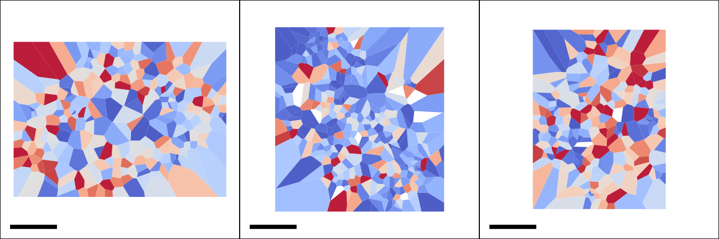
4.5. TRamWAy analysis

TRamWAy is a cutting-edge analysis tool for single molecule dynamics such as diffusivity and potential energy spatiotemporally. (Laurent et al., 2022). TRamWAy is provided as a python package tramway.

Slitflow provides wrapping classes of some of the helper functions in the tramway package, including tessellation, inference, and map_plot.

The following example calculates and visualizes the spatial map of molecular diffusivity for each cell nucleus.

PL = sf.manager.Pipeline(project_dir)

PL.add(sf.trj.wtramway.Tessellation(), 1, (5, 1), "tram", "tess",
       ["RPB1"], [(1, 10)], [1], {"method": "gwr", "split_depth": 1})
PL.add(sf.trj.wtramway.Inference(), 0, (5, 2), None, "infer",
       ["RPB1"], [(5, 1)], [1], {"mode": "d"})
PL.add(sf.trj.wtramway.MapPlot(), 2, (5, 3), None, "map",
       ["RPB1"], [(5, 1), (5, 2)], [1, 1],
       {"feature": "diffusivity", "param": {"unit": "std"}})
PL.add(sf.fig.style.Basic(), 0, (5, 4), None, "fig_style",
       ["RPB1"], [(5, 3)], [1],
       {"size": [4, 4], "margin": [0, 0, 0, 0], "is_box": True,
       "limit": [-14, 14, -14, 14], "tick": [[-15, 15], [-15, 15]],
        "clim": [0, 0.06], "cmap": "coolwarm"})
PL.add(sf.fig.figure.ToTiff(), 0, (5, 5), None, "fig_tif",
       ["RPB1"], [(5, 4)], [1],
       {"scalebar": [5, 0.05, 0.05, 2, [0, 0, 0]],
       "dpi": 300, "split_depth": 0})
PL.add(sf.img.montage.RGB(), 0, (5, 6), None, 'fig_mtg',
       ["RPB1"], [(5, 5)], [0],
       {"grid_shape": [1, 3], "padding_width": 0, "split_depth": 0})
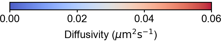
PL.add(sf.fig.style.ColorBar(), 0, (5, 7), None, "colorbar",
       ["RPB1"], [(5, 4)], [1],
       {"tick": [0, 0.02, 0.04, 0.06], "format": "%0.2f"})
PL.add(sf.fig.figure.ToTiff(), 0, (5, 8), None, "cb_tif",
       ["RPB1"], [(5, 7)], [1], {"split_depth": 1})

PL.save("pipeline_6_tramway")
PL.run()

4.6. Make pipeline flowchart

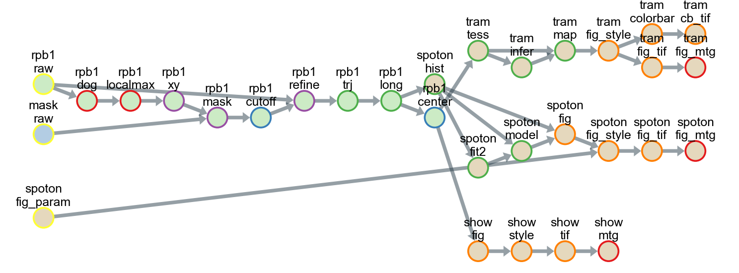
All tasks, including tracking, analysis, and drawing, can be saved as a single pipeline script text file in the CSV format for reuse and distribution. Using the pipeline script, a series of data-processing steps from the raw data to the final image could be exported as a flowchart.

Each circle in the flowchart represents an individual task corresponding to an analysis subfolder in the project directory. The arrows between circles represent data dependencies. In this example, 26 different classes were used, and all the data were stored in 31 subfolders in five groups.

The flowchart can be created with the following script:

PL = sf.manager.Pipeline(project_dir)

PL.load(["pipeline_1_load", "pipeline_2_tracking",
         "pipeline_3_show_trajectory", "pipeline_4_spot_on",
         "pipeline_5_spot_on_figure", "pipeline_6_tramway"])

PL.make_flowchart("pipeline", "grp_ana", scale=(0.6, 1.8))