Basic usage
This short example of Slitflow usage enables us to overview Slitflow by analyzing the trajectories of simulated random walks.
Installation
Slitflow can be installed from PyPI.
pip install slitflow
This command will install minimal dependencies for basic usage. Some analysis class requires additional packages. To install all required packages, see also the detailed installation guide.
We usually import slitflow as follows:
import slitflow as sf
Simulate random walks
Start by creating an Index object that defines the number of images and
trajectories. Then we execute the run() method to make result data inside
the Index object.
See also slitflow.tbl.create.Index for argument descriptions.
D1 = sf.tbl.create.Index()
D1.run([], {"type": "trajectory", "index_counts": [2, 3], "split_depth": 0})
print(D1.data[0])
#   img_no trj_no
# 0      1      1
# 1      1      2
# 2      1      3
# 3      2      1
# 4      2      2
# 5      2      3
Then we append random walk coordinates to the index table by making the next analysis object.
See also slitflow.trj.random.Walk2DCenter for argument descriptions.
D2 = sf.trj.random.Walk2DCenter()
D2.run([D1], {"diff_coeff": 0.1, "interval": 0.1, "n_step": 5, "length_unit": "um", "seed": 1, "split_depth": 0})
print(D2.data[0])
#    img_no  trj_no  frm_no      x_um      y_um
# 0        1       1       1  0.000000  0.000000
# 1        1       1       2  0.229717 -0.325487
# 2        1       1       3  0.143202 -0.078733
# 3        1       1       4  0.068507 -0.186384
# 4        1       1       5 -0.083234 -0.141265
# ...
# 34       2       3       5 -0.218346  0.373677
# 35       2       3       6 -0.247888  0.498855
Calculate the Mean Square Displacement
The following code calculates the MSD of each trajectory. Then MSDs are averaged through all images.
See also slitflow.trj.msd.Each and slitflow.tbl.stat.Mean.
D3 = sf.trj.msd.Each()
D3.run([D2], {"group_depth": 2, "split_depth": 0})

D4 = sf.tbl.stat.Mean()
D4.run([D3], {"calc_col": "msd", "index_cols": ["interval"], "split_depth": 0})
print(D4.data[0])
#    interval       msd       std       sem  count       sum
# 0       0.0  0.000000  0.000000  0.000000      6  0.000000
# 1       0.1  0.034335  0.014093  0.005754      6  0.206012
# 2       0.2  0.065532  0.023673  0.009665      6  0.393195
# 3       0.3  0.116515  0.031346  0.012797      6  0.699089
# 4       0.4  0.138391  0.066066  0.026971      6  0.830347
# 5       0.5  0.153488  0.112978  0.046123      6  0.920926
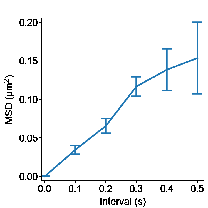
Make a figure image
Then plot the averaged MSD against the time interval. The graph style is adjusted using style class and creates a figure tiff image.
See also slitflow.fig.line.Simple, slitflow.fig.style.Basic and slitflow.fig.figure.ToTiff
import matplotlib.pyplot as plt

D5 = sf.fig.line.Simple()
D5.run([D4], {"calc_cols": ["interval", "msd"], "err_col": "sem", "group_depth": 0, "split_depth": 0})

D6 = sf.fig.style.Basic()
D6.run([D5], {"limit": [-0.01, 0.52, -0.005, 0.205], "tick": [[0, 0.1, 0.2, 0.3, 0.4, 0.5], [0, 0.05,
      0.1, 0.15, 0.2]], "label": ["Interval (s)", "MSD (\u03bcm$^{2}$)"], "format": ['%.1f', '%.2f']})

D7 = sf.fig.figure.ToTiff()
D7.run([D6], {"split_depth": 0})

plt.close()
plt.imshow(D7.to_imshow(0))
plt.axis("off")
plt.show()
Run using pipeline
The Pipeline class can perform all the above steps while saving data to a project folder.
import os

# make a project directory (in the user directory)
prj_dir = os.path.join(os.path.expanduser("~"),"slitflow","tutorial_pipeline")
if not os.path.isdir(prj_dir):
   os.makedirs(prj_dir)
print(prj_dir)

# make and run a pipeline
PL = sf.manager.Pipeline(prj_dir)
obs_names = ["Sample1"]
PL.add(sf.tbl.create.Index(), 0, (1, 1), 'channel1', 'index',
      obs_names, [], [],
      {"type": "trajectory", "index_counts": [2, 3], "split_depth": 0})
PL.add(sf.trj.random.Walk2DCenter(), 0, (1, 2), None, 'trj',
      obs_names, [(1, 1)], [0],
      {"diff_coeff": 0.1, "interval": 0.1, "n_step": 5, "length_unit": "um", "seed": 1, "split_depth": 0})
PL.add(sf.trj.msd.Each(), 0, (1, 3), None, 'msd',
      obs_names, [(1, 2)], [0],
      {"group_depth": 2, "split_depth": 0})
PL.add(sf.tbl.stat.Mean(), 0, (1, 4), None, 'avemsd',
      obs_names, [(1, 3)], [0],
      {"calc_col": "msd", "index_cols": ["interval"], "split_depth": 0})
PL.add(sf.fig.line.Simple(), 0, (1, 5), None, 'msd_fig',
      obs_names, [(1, 4)], [0],
      {"calc_cols": ["interval", "msd"], "err_col": "sem", "group_depth": 0, "split_depth": 0})
PL.add(sf.fig.style.Basic(), 0, (1, 6), None, 'msd_style',
      obs_names, [(1, 5)], [0],
      {"limit": [-0.01, 0.52, -0.005, 0.205], "tick": [[0, 0.1, 0.2, 0.3, 0.4, 0.5], [0, 0.05, 0.1, 0.15, 0.2]],
      "label": ["Interval (s)", "MSD (\u03bcm$^{2}$)"], "format": ['%.1f', '%.2f']})
PL.add(sf.fig.figure.ToTiff(), 0, (1, 7), None, 'msd_img',
      obs_names, [(1, 6)], [0],
      {"split_depth": 0})
PL.save("pipeline")
PL.run()
This code creates the following folder structure.
tutorial_pipeline
 |--g0_config
 |    pipeline.csv
 |--g1_groupe1
     |--a1_index
     |    Sample1_index.csv
     |    Sample1_index.sf
     |    Sample1_index.sfx
     |--a2_trj
     |    Sample1_trj.csv
     |    Sample1_trj.sf
     |    Sample1_trj.sfx
     |--a3_msd
     |    Sample1_msd.csv
     |    Sample1_msd.sf
     |    Sample1_msd.sfx
     |--a4_avemsd
     |    Sample1_avemsd.csv
     |    Sample1_avemsd.sf
     |    Sample1_avemsd.sfx
     |--a5_msd_fig
     |    Sample1_msd_fig.fig
     |    Sample1_msd_fig.sf
     |    Sample1_msd_fig.sfx
     |--a6_msd_style
     |    Sample1_msd_style.fig
     |    Sample1_msd_style.sf
     |    Sample1_msd_style.sfx
     |--a7_msd_img
          Sample1_msd_img.tif
          Sample1_msd_img.sf
          Sample1_msd_img.sfx
We can use the make_flowchat() method of the pipeline object to create an analytical flowchart diagram. The image is created as a PNG file in the g0_config folder in the project directory.
PL.make_flowchart("pipeline", "grp_ana")
